How to Use KineMaster in 3 Easy Steps

If you like making videos for social media or from family events, KineMaster is here to help. It’s an editing app that’s easy to use and won’t break your bank. It offers two subscription models (monthly and annual pricing) with a 7-day trial.

Let’s see what this application has to offer.

  1. Import media

    How to Use KineMaster

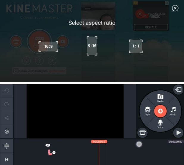
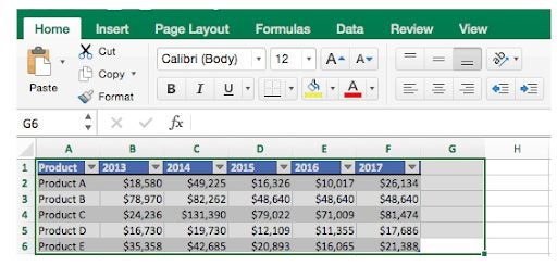
    When you first open the application, it asks you to choose the ratio of the final product. Afterwards, you can click the “Media” icon to import files from your local or cloud storage. Once the timeline is inhibited with material, you can start editing.

  2. Edit the video

    How to Use KineMaster

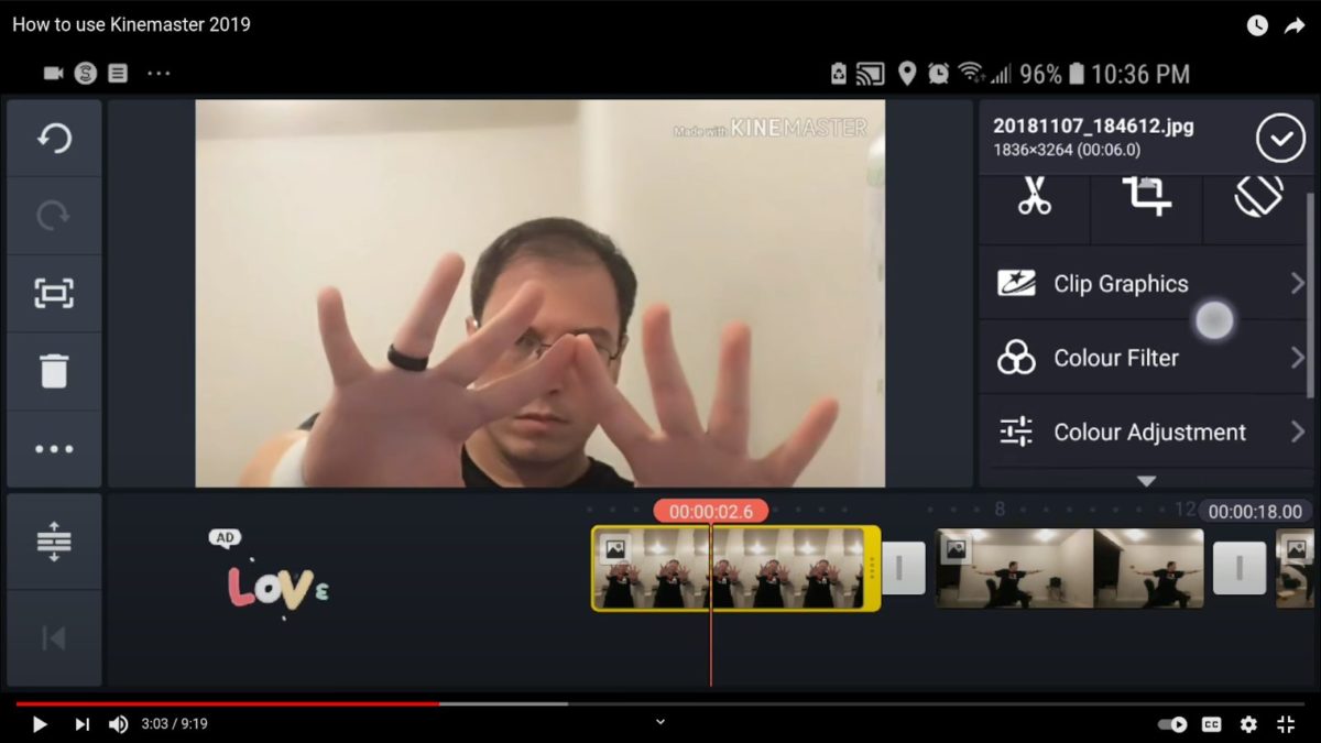
    This app allows you to trim, arrange, and layer visuals, remove the voice, add audio, and so much more! Each clip can be modified in a myriad of ways, from color correction to overlay. The reverse tool lets you rewind the video, make focal shifts, and add transitions.

  3. Export and share

    How to Use KineMaster

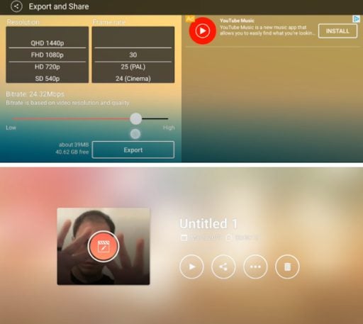
    The app allows you to export the product in 4K 60fps, saving it on the device or in the cloud storage of your choice. You can also backup the videos directly in the application and share them anywhere, including YouTube, messenger apps, and social media.

Features to dazzle!

We’ve already talked about the reverse and blending modes above. They let you have creative and artistic solutions in your everyday videos. Still, there’s so much more to explore in KineMaster!

The paid version includes all the mentioned features, plus access to the KineMaster Asset Store. It lets you get music, fonts, stickers, and effects. At the same time, the ready projects make it easier to add your video material over templates.

Microsoft Excel: How to Freeze a Row in 2 Fast Methods

Reading large spreadsheets can get tricky, as the usual drill requires you to keep the first few rows or columns frozen for easier use. However, you don’t have to call Sub-Zero to freeze rows in Excel.

Our article gives you a few other, less menacing methods.

  1. Freeze top row or first column

    How to Freeze a Row

    Excel’s functionality includes the first row and first column freezing as a default in the “Freeze Panes” dropdown menu. To access it, you need to go to the spreadsheet, click the “View” menu, navigate to “Freeze Panes,” and click the arrow.

    You’ll see three choices. The bottom two are referring to the “First Row” and “First Column.” You can choose one, the other, or both.

  2. Fix rows and columns

    How to Freeze a Row

    There might be cases where freezing the first row and column isn’t enough. To ensure convenience, you can also suspend more than one of them. To freeze more than one row, follow the steps below:

    – Click the row below what you want visible at a scroll

    – Go to View > Freeze Panes

    – Choose the top option

    The same trick works for the columns:

    – Click a column to the right of what you want frozen

    – Go to View > Freeze Panes

    – Click the unspecified panes option on top of the list

    You can also halt columns and rows at the same time. Just click a tile, and go to the “Freeze Panes” selection mentioned above. Once you click, all the rows above and columns to the left of the selected tile will stay in place.

Melt the ice

Once you have a row or a column frozen in a worksheet, the mentioned menu will add an “Unfreeze Panes” option. If you want to “melt” the rows, just click it, and it’ll unlock all the columns and rows.

How to Unlock Microsoft Excel in 3 Steps

Microsoft Excel is a giant in the industry when it comes to storing, manipulating, and presenting data on your Windows or Mac computer. There may be some cases where the data you are working with is confidential, such as financials, password logs, personal details, and more.

As such you may need to apply more security by locking Excel spreadsheets that contain sensitive information. However once the spreadsheet has been protected, how do you unlock it when you need to work on the file? Let’s look at how you can unlock a Microsoft Excel protected worksheet.

  1. Open the Spreadsheet

    How to Unlock Microsoft Excel

    First off, you will need to open the spreadsheet that you need to work on. You can do this by double-clicking on the file on your computer, or by opening the file directly from Excel.

  2. Unprotect Sheet

    How to Unlock Microsoft Excel

    Protected worksheets display a padlock icon next to the tab name in the bottom control panel of Excel. Right-click on the sheet with the padlock to open the context menu with further options. Similarly, if certain cells or ranges of data have been locked they will also show a padlock when hovering over the cells.

    In the context menu that appears in the top ribbon of Excel, click on ‘Unprotect Sheet’. If no password was set the file will open automatically. If there was a password set for added protection, move to the next step.

  3. Insert Password

    How to Unlock Microsoft Excel

    If the worksheet is protected with a password, a window will pop up asking you to input the password. Type in the password and click on ‘Ok’. If the password is correct, the protected worksheet will open.

    Be aware that users can protect whole worksheets or even just certain cells or ranges of data within a spreadsheet, but the method of unlocking remains the same.

Keep Sensitive Information Safe, Secure, and Well Protected in Excel

Microsoft Excel makes it easy to keep your confidential information protected by providing options to lock worksheets with passwords. Unlocking is a simple process if you have the right permissions or password on hand.

How to Convert Microsoft Excel to Google Sheets in 3 Simple Steps

The battle between Excel and Google Sheets carries on between these two spreadsheet giants. Although both programs work very similarly, users usually prefer one or the other on their Windows or Mac computers. 

But what happens if you need to send an Excel file to a Google Sheets user? Or vice versa? Luckily it is a relatively simple process to convert Excel to Google Sheets. Let’s see how you can do it below.

  1. Upload File

    How to Convert Microsoft Excel to Google Sheets

    Open your Google Drive on your computer. You can navigate to Google Drive from the grid icon in Gmail, or by typing drive.google.com in your search bar. Next, you need to upload:

    – In the top-left of the screen click on the + icon and choose ‘File Upload’ from the dropdown list.

    – Select the Excel file you want to upload from your computer.

  2. Open the Excel File

    How to Convert Microsoft Excel to Google Sheets

    – Double-click on the Excel file in your Drive. This will only open a preview of the Excel spreadsheet. – Click on ‘Open with Google Sheets’ at the top of the screen.

  3. Save as Google Sheets

    How to Convert Microsoft Excel to Google Sheets

    Now that your Excel file is open in Google Sheets, you can save it as a Sheets file. 

    – Click on ‘File’ in the top menu.

    • Scroll down and choose ‘Save as Google Sheets’.

Collaborate on Spreadsheet Across Excel and Google Sheets

Now you can work on, send and collaborate on this spreadsheet regardless of whether you or your colleague has Excel.

Remember however that any changes made on the Google Sheets spreadsheet will not automatically appear on the Excel sheet as well. To use the latest Sheets spreadsheet in Excel you will need to download the sheet in Excel format from your Drive. To do this, you simply highlight the spreadsheet in Drive, then right-click on it and select ‘Download’ and choose the Excel format.

How to Use Microsoft Excel Formulas in 3 Simple Steps

Have you started working in Microsoft Excel? If you have, then formulas might still seem a little intimidating to you, but they are actually very useful and if you keep a few simple things in mind, can even be easy to use.

Excel is very useful for storing, manipulating, and presenting various forms of data on your Windows or Mac computer. Excel has a useful formula wizard that can assist you in using various functions.

  1. Access the Formula Wizard

    How to Use Microsoft Excel Formulas

    When you are in your spreadsheet, click on the cell you want to enter the formula into and type =. Formulas always start with a =. Next click on the formula icon in the top bar represented by the fx symbol.

  2. Choose the Formula

    How to Use Microsoft Excel Formulas

    The next window will show the available functions. You can choose your formula from the list if you already know what it is, or you can type the description into the box and see which formula Excel recommends.

  3. Insert Function Arguments

    How to Use Microsoft Excel Formulas

    You will be taken to a new window, sometimes called the formula palette, where you have to input the data from your spreadsheet. The wizard tells you what information needs to be inserted. 

    – Next to the argument click on the grid icon with the red arrow to be taken to your spreadsheet.

    • Select the data from the cells in your spreadsheet.

    The formula palette will show you a description of the formula in the window, as well as an example of the formula and the result at the bottom so that you can check your information easily.

Use Formulas Confidently

By using the formula wizard in Excel you can learn to use formulas right from the start with a good helping hand. Soon you’ll be using the formulas without even needing the wizard.

Among Us Hits The Epic Store for Free!

You Can Now Play Among Us For Free On The Epic Store

Among Us has been available for PC for some time now, but it’s only been free for mobile gamers. It’s led to many players installing Android emulators like BlueStacks to avoid paying for the Windows version. Well, times are changing. Epic Store has announced that you can now grab the social detection game for no charge at all.

There’s one catch, though. The sale is only live until June 3, 2021, which means you’ll have to move quickly to get your hands on it. The price will return to normal after that, but it only includes the base game and not any of the extras.

Among Us Hits The Epic Store for Free!

This Mega Sale is part of Epic Store’s latest promotional campaign to bring more players to the platform. Every Thursday, there will be a new free game for you to download as long as you’re a registered member. This month started with NBA 2K21 as the free gift, which is a massive title to simply give away.

If you’re keen on downloading Among Us for free, you need to head to the Epic Store sale page. You’ll see the promotion on the page, but you’ll need to register for an account first if you don’t have one. From there, install the gaming client before you proceed to download the game. You’ll see it appear on the client, ready for you to hunt down your friends silently.

How to Update Microsoft Excel in 2 Methods

Although the subscription model is rising, some users still have the installed version of Excel. Microsoft still supports the software by sending updates from time to time. If you’re one of the lucky people that bought the app previously, read on to learn how to update it.

  1. On Windows

    How to Update Microsoft Excel

    Updating Excel is super easy and can be accomplished in a few clicks. Here are the steps you can take:

    – Open the program

    – Go to the “File” menu

    – Indicate if updates are available

    – Click “Update Options”

    – Select “Update Now”

    – Wait until they install

  2. On Mac

    How to Update Microsoft Excel

    If you own a MacOS device, the process is as follows:

    – Open Excel

    – Go to Help

    – Select the “Check for Updates” option

    – Click the “Automatically Download and Install” choice

    – Select the “Check for Updates” to initiate the download

    • Wait until the new version settles, and the program restarts

Can you activate automatic updates?

The automatic updates on Office apps, including Excel, are allowed only on Mac. Go to the “Updates” page on your Mac, as described above, and check the “Automatically keep the Microsoft Apps up to date” box. If you’ve downloaded the program from the App Store, go to the “Updates” page and click “Update All.” You can also open the beta channel to get the latest and greatest features before anyone else.

How to Download Microsoft Excel in 3 Easy Methods

Excel is the industry-leading spreadsheets-management software the majority of Windows users still prefer. While you can buy the program outright, there are other options to explore as well.

Let’s see how you can get the latest version of the application.

  1. Good-old licensed software

    How to Download Microsoft Excel

    Buying the licensed software has been the only way to go for decades. If you’re one of those who still prefer owning your programs and not worrying about subscriptions, this option is for you. An upfront fee, a couple of clicks in the “Installation Wizard,” and the program will be on your PC or Mac, serving you forever.

    Microsoft still issues updates to the software.

  2. Subscribe to Microsoft 365

    How to Download Microsoft Excel

    If you’re internet-bound and like your software on all your devices and web, subscribing to the Microsoft 365 program is a better solution. While you only get the program on one computer in the first method, the subscription gains you access to your documents in One Drive storage and other Office programs like Outlook, Word, and PowerPoint.

    It also offers Personal, Family, and Business plans, which have various functions and differ in price.

  3. Use a free trial

    How to Download Microsoft Excel

    If you’re not sure about the subscription offer or just want to see how the bundle works for your situation, use the free trial of the app bundle. You can access it from Microsoft’s official website.

The rise of the subscription model

Do you remember the days when you could buy a computer program for life and update it endlessly? These sunny days are in the past. While paying smaller fee installments monthly or yearly is convenient, some old-school users still prefer owning the applications. Sadly, most software manufacturers prefer the constant cash flow of the subscription model nowadays.

How to Make a Graph on Microsoft Excel in 4 Steps

Using Microsoft Excel on Windows and Mac is becoming one of the best ways to store, manipulate and analyze data. With many different features specifically for data analysis, it is easy to understand why the program is so popular.

One of the ways you can present your data is through the use of graphs and pie charts. This may sound complicated to do within a computer program, but fear not, Excel has made it a simple process.

  1. Enter Data Into the Spreadsheet

    How to Make a Graph on Microsoft Excel

    Before you can start to make a graph, you first need to have data available. In your Excel spreadsheet add the data that you want to create the graph for. Also, make sure to add clear headings to your columns and rows as this will be included in your graph’s axis and is needed to clearly understand what you are looking at.

  2. Select the Range of Data to Be Used in the Graph

    How to Make a Graph on Microsoft Excel

    Next, you need to highlight the data that you want to use in your graph. You can do this by clicking and dragging the mouse across the cells you want to use. Remember to include the headings.

  3. Choose Chart Type

    How to Make a Graph on Microsoft Excel

    With the data selected click on ‘Insert’ in the top ribbon, now navigate to the dropdown list of all the ‘Recommended Charts’ and choose the graph that will best represent your data from the various options. Once you’ve clicked on the chart type, the program will automatically generate your graph from the data you selected.

  4. Check and Improve Your Graph

    How to Make a Graph on Microsoft Excel

    Now that the graph has been generated you can check that the elements appear correct, and make adjustments such as the size of the graph, title of the graph and axis, change the colors used, and the display.

Creating Simple Graphs to Represent Data in Excel

With Excel, it is simple to create graphs to represent your data visually. Being able to use graphs is great when you need to present information to others as it makes the data easier to understand and visualize.

Microsoft Excel Tips – Top 4

Microsoft Excel is a popular spreadsheet program used to store, manipulate and analyze various forms of data. If you are using Excel on your Windows or Mac computer, you may be wondering how you can further optimize your skills using the program.

Here are a few tips to make your data analysis easier, and more professional.

  1. Use Conditional Formatting

    Microsoft Excel Tips

    Conditional formatting is a useful function that can highlight variances in your data so that they become immediately visible. To use conditional formatting you highlight the cells that you want to apply the formatting to, and then choose conditional formatting from the options in the ribbon. A window will open where you can set your criteria for the formatting.

  2. Paste Special

    Microsoft Excel Tips

    Copy and pasting are used often in Excel spreadsheets, but there are many different ways you can paste data. You can choose to just paste the text, the text and formulas, or even include the formatting. To choose the special formatting that you require, right-click on the cell where you will be pasting the data. Now, click on ‘Special Paste’ and there will be many options to choose from.

  3. Adding Multiple Rows

    Microsoft Excel Tips

    Sometimes you will get to a point where you need to add more rows to your spreadsheet. This is easy enough to do. Highlight an empty row at the bottom of the sheet where you want to add more, right-click and choose ‘Add Row’. If you want to add multiple rows, highlight a few rows and repeat the process.

  4. Absolute References

    Microsoft Excel Tips

    This is an indispensable tool when using Excel. Sometimes when you copy a formula it adjusts the formula to the next row or column, but you may not always want that. You may want a value in your formula to always refer to a certain cell or value. To do this you have to place a $ before the row reference and again before the column reference, for example, $A$10. This will lock the reference in the formula.

Learn to Master Excel With a Few Simple Tips

Learning to master Excel can take a while, but when implementing a few of these tips you’ll soon be on your way to creating masterful spreadsheets.